Introduction

MMVSola Predictor is a web tool for pharmacokinetic (PK), pharmacodynamic (PD), and dose prediction of malaria drug candidates. It estimates human PK/PD model parameters based on in vitro and in vivo animal experimental data, and simulates PK/PD profiles to predict minimal efficacious doses for oral and long-acting injectable (LAI) formulations. Human pharmacokinetics - clearance and volume of distribution - are predicted from in vitro metabolism data via in vitro-to-in vivo extrapolation (IVIVE) and/or from preclinical in vivo data via allometric scaling (Section 2.2). Human pharmacodynamics - the parasite-killing effect as a function of drug concentration - are predicted from in vitro parasite reduction ratio (PRR) and growth-inhibition assay data, and/or from SCID mouse EC₅₀ estimates (Section 2.3). These PK and PD parameters drive a combined PK/PD simulation (Section 2.1) from which the efficacious dose is derived (Chapter 3).

Input → Prediction → Report

MMVSola organizes its workflow into three steps, mirroring its three main tabs: Input → Prediction → Report

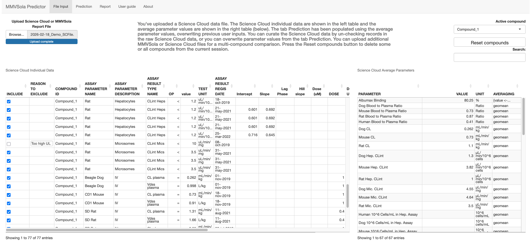
Input. From the File Input tab, the user provides in vitro and animal in vivo experimental parameters for one or more drug candidates (compounds), either by uploading a ScienceCloud database extract or a previously generated MMVSola Excel report. When data from multiple compounds have been uploaded, an Active compound select input allows to select the compound for which data will be displayed. When ScienceCloud data is available for the active compound, there can be several records for the same parameter (e.g. replicate assay measurements). These multiple measurements are averaged into a single input value. The user can review and exclude individual records from this averaging. Hovering the mouse over the Averaging cell reveals the expression used to derive the averaged value, in case it is too long to display in full.

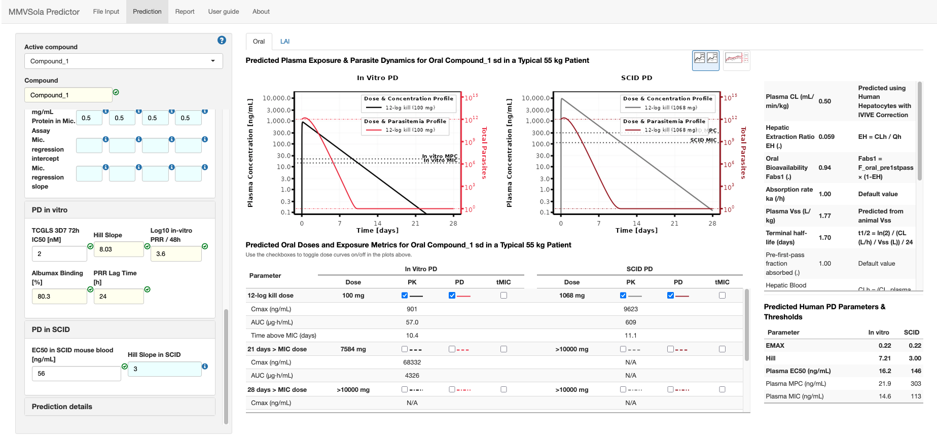
Prediction. The Prediction tab is a dashboard displaying, for the selected active compound, the validated input values - menu panel on the left and predictions - main panel. Each input field is colour-coded by its source:

azure: a default value calculated from other available inputs or taken from the literature;
gold: a compound-specific average derived from the uploaded experimental data;
white: a value entered (or overwritten) manually by the user.

See Chapter 1 for a guided tour of the input menu, including how MMVSola fills in missing values for you. The Oral and LAI tabs summarize the predicted human PK/PD parameters, the predicted doses, and the PK/PD profiles simulated at the predicted doses in a typical patient. The user can interactively explore how changing any input parameter and/or the simulated doses affects the predictions.

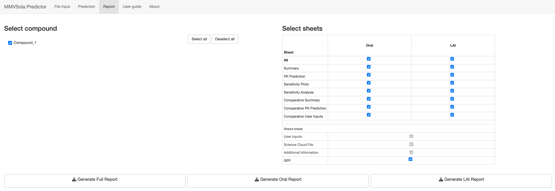
Report. The Report tab lets the user customize and download a multi-sheet Excel report documenting the inputs, the predicted PK/PD parameters and doses, and (when several compounds have been loaded) side-by-side comparison tables across candidate compounds. A previously generated MMVSola report can itself be re-uploaded as an input file, which makes it easy to pick up earlier work or to compile results from several sessions. See Section 4 for details on what each report sheet contains.

This user guide first walks you through a practical usage scenario (Chapter 1), then describes the underlying methods - human PK/PD parameter prediction (Chapter 2) and dose prediction (Chapter 3) - and finally explains how to make the most of the Report tab (Chapter 4) and covers a few more advanced topics (Chapter 5).

1 Quick Start

This chapter is a step-by-step guide to getting your first PK/PD prediction out of MMVSola. You will: name your compound, fill in what you know, let MMVSola fill in the rest, and read off the result.

A few tips before you start:

Screenshots appear blurred? Right-click any screenshot and choose Open image in new tab (or equivalent in your browser) to view it at full resolution.
Use a large screen. MMVSola is designed for a wide layout. On a smaller screen the panels may overlap or be cut off. If that happens, zoom your browser window out:
- Chrome / Edge / Opera: Ctrl + - (Windows/Linux) or Cmd + - (Mac); or click the three-dot menu → Zoom.
- Firefox: Ctrl + - / Cmd + -; or the three-line menu → Zoom.
- Safari: Cmd + -; or the View menu → Zoom Out.
Help icons. Blue circles with a question mark (ⓘ) appear throughout the MMVSola interface. Hovering the mouse pointer over one opens a help message explaining the corresponding input or panel.

Before you start: export the data from Science Cloud

If your compound is in Science Cloud, you can load its data instead of typing it in. Select your compounds and batches in Science Cloud, click Export above the results table (Figure 1.1), choose RD-00-0000 - GENERIC MMVSOLA EXTRACTION on the Standard tab and click Export again (Figure 1.2). The Excel file this produces can be uploaded on the File Input tab.

Figure 1.1: The Export button in the Science Cloud search results

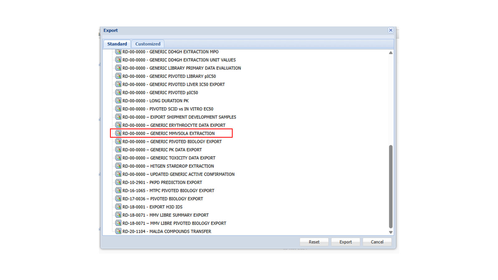
Figure 1.2: The Science Cloud export dialog with the extraction to select highlighted

Step 1: Name your compound and open an input group

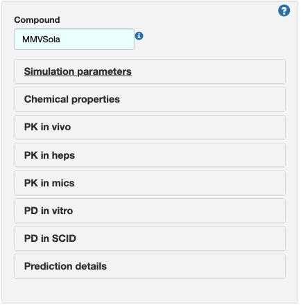
After loading the app, enter a name in the Compound field (or keep the default MMVSola). Below it is a list of collapsible input groups - Simulation parameters, Chemical properties, PK in vivo, PK in heps, PK in mics, PD in vitro, PD in SCID, and Prediction details. Click on an input group title to expand it and reveal its input fields.

Step 2: Simulation parameters

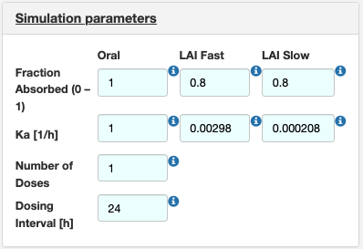
Open Simulation parameters to set the dosing regimen and absorption inputs for the Oral and LAI (long-acting injectable) routes: fraction absorbed, absorption rate constant (\(k_a\)), number of doses, and dosing interval. MMVSola pre-fills these with sensible defaults (shown on an azure background) that you can overwrite at any time.

Step 3: Chemical properties

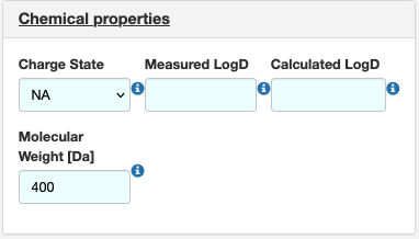
Open Chemical properties and enter the compound’s charge state, LogD (measured or calculated), and molecular weight. These values feed into several of the predictions described in the 2 chapter, for example the conversion of in vitro IC₅₀ values from nM to µg/mL.

Step 4: PK in vivo

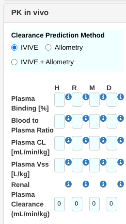
Open PK in vivo to choose the clearance prediction method (IVIVE, Allometry, or IVIVE + Allometry, see Section 2.2.3) and enter plasma binding, blood-to-plasma ratio, plasma clearance, plasma volume of distribution (V_ss), and renal plasma clearance for human (H), rat (R), mouse (M), and dog (D), as available. Unlike the other columns, human (H) Plasma CL and Plasma Vss have no ScienceCloud filter, since they can only be calculated from other inputs or entered manually - if you have a known human value (e.g. from clinical PK data), enter it directly here and it overrides the predicted value everywhere downstream, exactly like any other manual entry.

Step 5: PK in heps and PK in mics

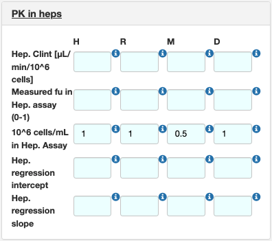
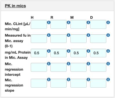
Open PK in heps and PK in mics to enter the in vitro metabolism data that drive the IVIVE clearance prediction: intrinsic clearance (CL_int), the unbound fraction measured in the assay, the assay scaling factor (10⁶ cells/mL for hepatocytes, mg protein/mL for microsomes), and, if available, regression correction parameters for a specific laboratory’s assay (see Section 2.2.3, Step 3).

Step 6: PD in vitro and PD in SCID

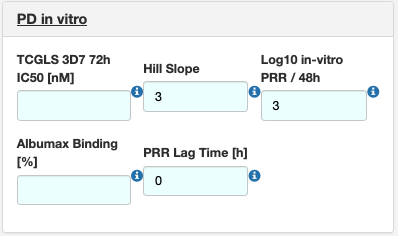
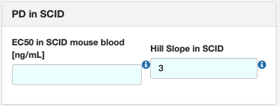
Open PD in vitro to enter the growth-inhibition assay IC₅₀ and Hill slope, the in vitro parasite reduction ratio (PRR) and its lag time, and the Albumax binding of the assay medium. For this walkthrough, enter 87 for Albumax Binding [%]. Open PD in SCID to enter an EC₅₀ and Hill slope measured directly in the SCID mouse model, if available. MMVSola uses whichever of these two data sources you provide - or both - to predict the PD parameters described in Section 2.3.

Step 7: Prediction details

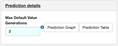
Open Prediction details to set the maximum number of “default value generations” (see Step 8 below) and to switch the result view between Prediction Graph and Prediction Table.

Step 8: Let MMVSola fill in the gaps

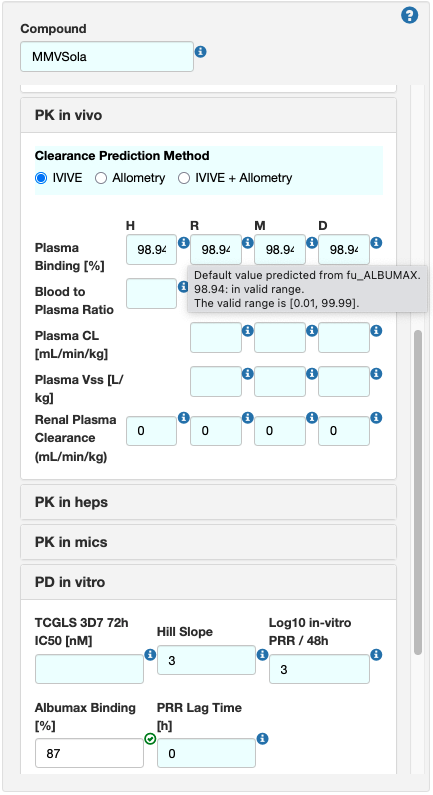
You do not need to fill in every field by hand. Whenever a value is missing, MMVSola tries to predict it from the inputs you have provided, and shows the result on an azure background. Hover over the blue i icon next to a field to see where its value came from and whether it is in the valid range.

For example, the Albumax Binding [%] entry of 87% entered in Step 6 is converted to an unbound fraction fu_ALBUMAX = 0.13, which MMVSola then uses as the starting point for predicting all other unbound fractions (see Section 5.2). The result for human Plasma Binding [%] - predicted from fu_ALBUMAX - is shown on an azure background, and the tooltip explains that the shown value (98.94%) was “predicted from fu_ALBUMAX”:

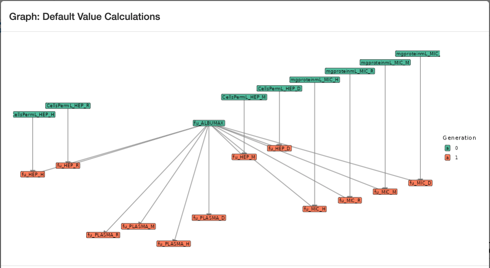
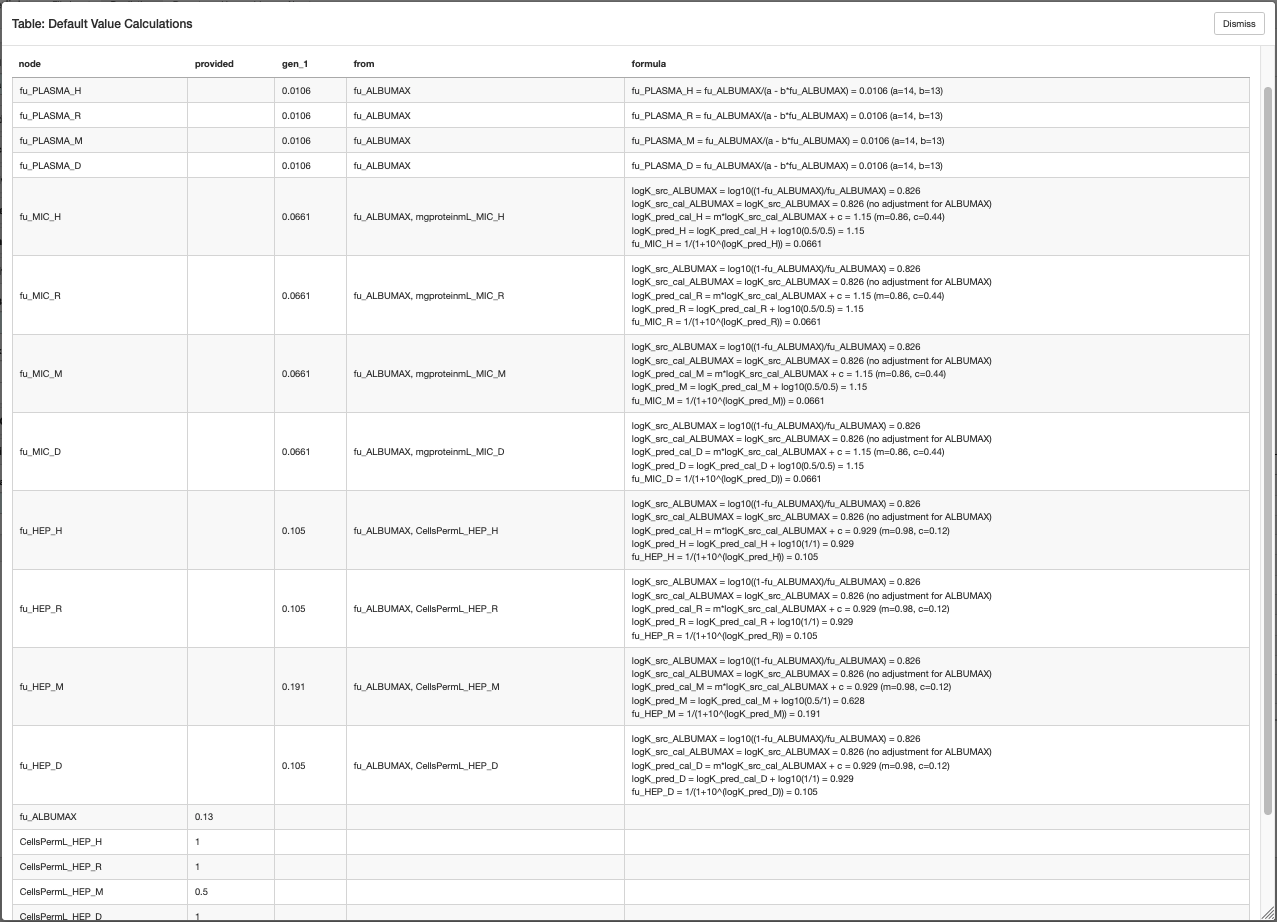
This chaining of predictions can go several levels deep (the Max Default Value Generations field from Step 7 limits how deep). The Prediction Graph and Prediction Table buttons under Prediction details let you inspect exactly which values were derived from which: the graph shows the dependency chain (e.g. fu_ALBUMAX → fu_HEP_* / fu_MIC_* → fu_PLASMA_*), and the table lists, for every derived parameter, the inputs and the formula used to calculate it.

Step 9: Follow the “still need to enter” guidance and view your prediction

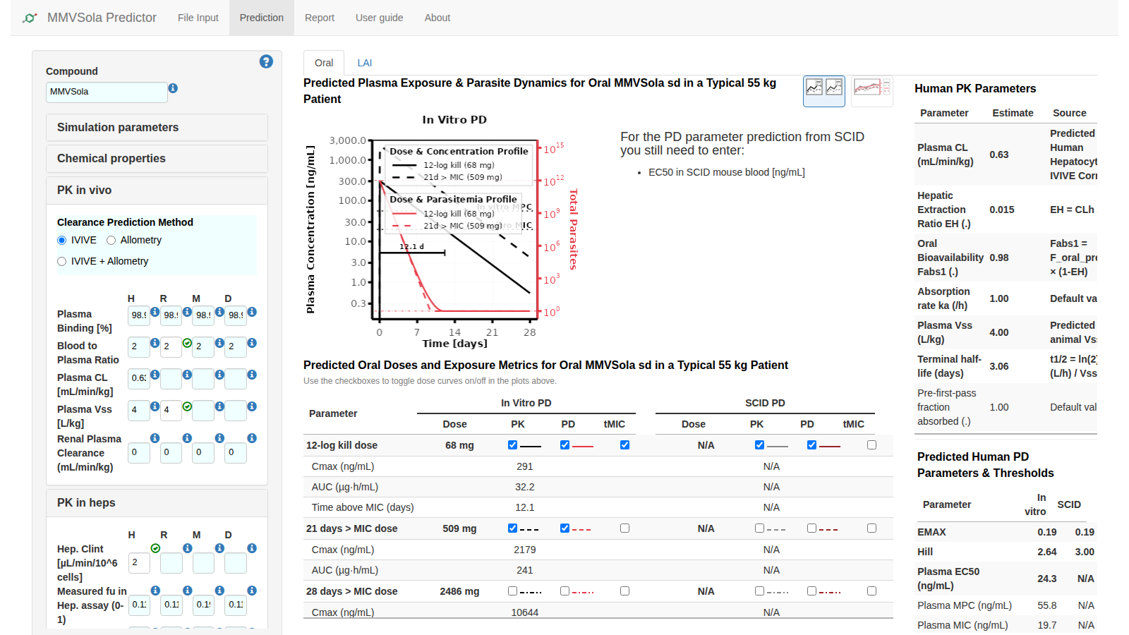
Switch between the MMVSola’s Oral or LAI tab. If any inputs required for the PK or PD prediction are still missing, MMVSola tells you exactly what they are, e.g. “For the PD parameter prediction from SCID you still need to enter: EC50_SCID”. For this walkthrough, enter the values shown with a white background in the screenshot below: Rat Blood to plasma ratio = 2, Human Hep CLint = 2, and TCGLS 3D7 72h IC50 = 2. This will result in Oral and LAI dose predictions and visualization of the PK/PD profiles for the top-most dose criteria in the Oral and LAI sub-tabs on the right. Then tick the checkboxes as shown to overlay the simulated PK/PD profile for the 21 days > MIC dose and the tMIC coverage segment for the 12-log kill dose on the plot above the table.

Step 10: Oral and LAI dose prediction

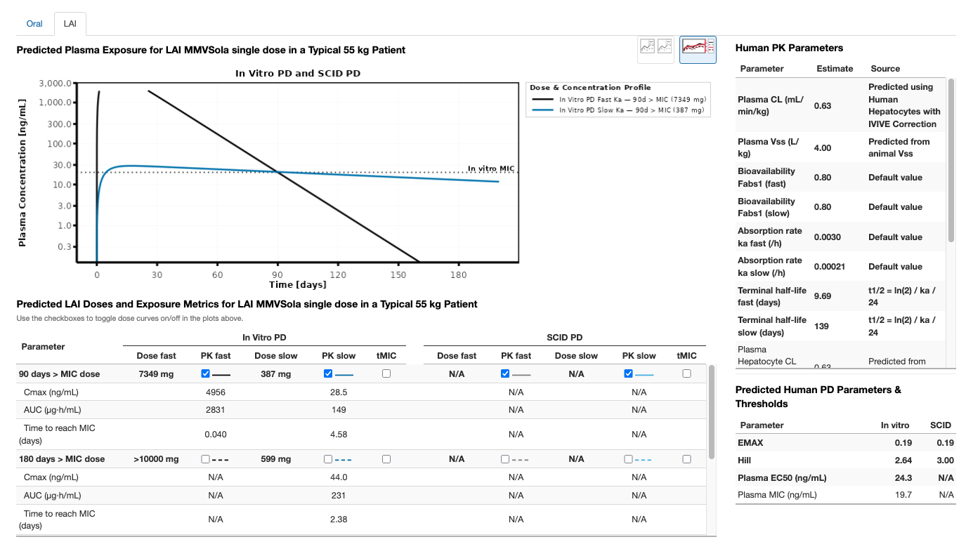
The Oral tab shows the predicted PK/PD profile and dose recommendations for short treatment courses and oral chemoprevention regimens (Section 3.1). The LAI tab does the same for long-acting injectable formulations (Section 3.2) - and needs a few additional inputs to configure the LAI simulation, described below.

MMVSola simulates the pharmacokinetics (PK) of LAI compounds using the same one-compartment model with first-order absorption and linear elimination as for oral dosing - clearance and volume are predicted with the same approach described in Section 2.2. To run an LAI simulation, define the bioavailability in the fraction absorbed fields of the Simulation Parameters input group (default: 80%) - since there is no first-pass metabolism for LAI dosing, the LAI bioavailability is equal to the fraction absorbed.

You will also need to enter one or more absorption rate constants (\(k_a\), 1/h) in the LAI fast and LAI slow fields. Two reference values are provided, based on known human absorption rates for medroxyprogesterone acetate (fast) and levonorgestrel butanoate (slow). If available, rat and dog \(k_a\) values can also be entered. Future versions of MMVSola are expected to support direct upload of rat and dog \(k_a\) values from ScienceCloud, with automatic assignment to the fast/slow fields and updated reporting labels.

Animal \(k_a\) values can be estimated from intramuscular (IM) PK studies using the log-linear terminal slope - often reported as lambda-z - assuming flip-flop kinetics, where \(k_a\) is approximately equal to that terminal slope. Alternatively, \(k_a\) can be estimated using population PK modelling of the animal data.

Once these inputs are provided, the LAI tab shows the simulated PK/PD profile and the predicted doses (Section 3.2). As on the Oral tab, the dose table lists each predicted dose with its own checkbox and an editable Dose field: ticking a row overlays its simulated profile and its tMIC coverage segment - a horizontal bar marking the onset and duration of the last uninterrupted period during which plasma concentrations stay above the MIC (Section 3.3), labelled with the resulting coverage in days (e.g. “92.4 d”) - on the plot above, while typing a different value into Dose immediately re-simulates and redraws that row, making it easy to explore “what dose would be needed to achieve N days of coverage?” without leaving the page. Switch from the Oral to the LAI sub-tab to see the corresponding LAI predictions.

Step 11: Generate and upload an MMVSola report file

Navigate to the Report tab and click Generate Full Report. Report generation takes about a minute; once the download starts, save the file. Open the report file in Excel and look at the Oral and LAI summary sheets. The plots shown there reflect the checkbox selection you did in Step 9.

To demonstrate the save-and-resume workflow, upload the same report you just downloaded back into the app: go to File Input, click Browse, and select the report file. Because a compound with the same name is already loaded, MMVSola will show a dialog notifying you that the uploaded compound was renamed with a suffix:

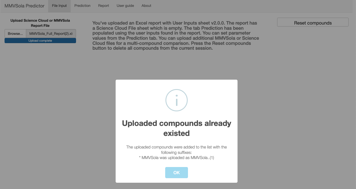
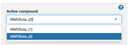
Click OK to confirm. If you kept the default compound name (MMVSola), the first upload renames it to MMVSola..(1). Upload the same report file a second time to create a copy named MMVSola..(2) - you will use this in Step 12.

Step 12: Comparing predictions across compounds

In the Active compound dropdown at the top of the left panel, select MMVSola..(2):

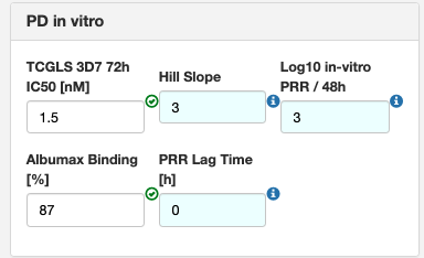
Open PD in vitro and change the TCGLS 3D7 72h IC50 [nM] value to 1.5. This gives the second compound a more potent in vitro profile, which will result in smaller predicted doses:

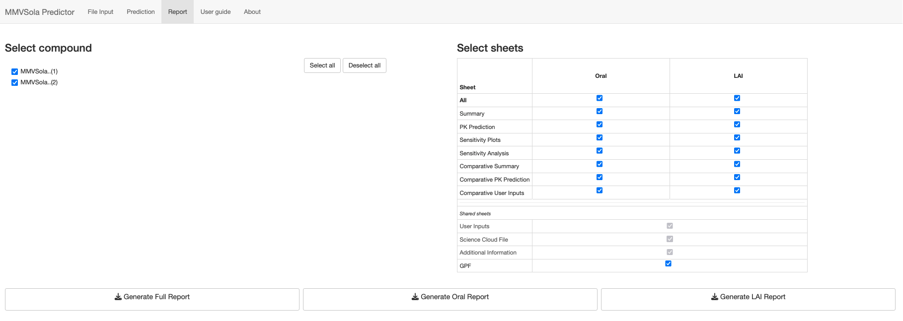
Now navigate to the Report tab. Both MMVSola..(1) and MMVSola..(2) should be ticked under Select compound - if not, tick them both (or click Select all). Then click Generate Full Report:

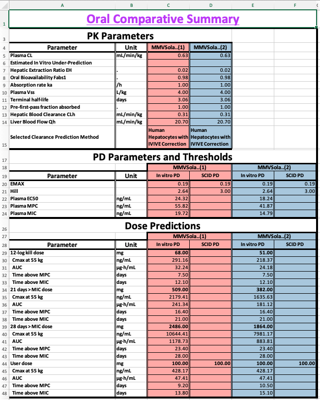
Open the downloaded workbook and navigate to the Oral Comparative Summary or LAI Comparative Summary sheet to see the two compounds side by side - comparing their plasma EC₅₀, PD thresholds, and predicted doses at a glance:

2 Human PK/PD Parameter Prediction

This chapter describes how MMVSola predicts human pharmacokinetic (PK) and pharmacodynamic (PD) parameters from experimental data, and how those parameters are used to simulate drug concentration and antimalarial activity over time.

2.1 Assumed Human PK/PD Structural Model

MMVSola uses a one-compartment pharmacokinetic model to describe how a drug moves through the body, combined with a parasite killing (PD) model to simulate the time-course of antimalarial activity.

The one-compartment model treats the entire body as a single, well-mixed pool. After dosing, drug is absorbed from the gut (or from the injection depot for LAI) at a rate governed by the absorption rate constant \(k_a\) and enters the bloodstream. From there, it is cleared at a rate described by the clearance CL relative to the apparent volume of distribution \(V_c\).

The PD model describes how fluctuating drug concentrations in the plasma drive changes in parasitemia (the number of circulating parasites). Without drug, parasites multiply exponentially, parameterized at the ln-parasitemia scale by a constant growth-rate (GR). When drug is present, it exerts a killing effect that follows a sigmoidal curve: the effect is half-maximal at the \(EC_{50}\) concentration, the maximum possible kill rate is \(E_{MAX}\), and the Hill coefficient (h) determines how steeply the effect increases with concentration. A PD lag time (\(k_{lag}\)) can be included to capture a delay between drug exposure and onset of killing - for example, a drug whose mechanism only becomes lethal once an exposed parasite reaches a specific stage of its ~48-hour life cycle, so that the killing effect of a given exposure only manifests some time later.

Body weight scaling. Clearance scales with body weight raised to the power 0.75 (\(CL \propto BW^{0.75}\)) and volume scales linearly with body weight (\(V_c \propto BW\)). The patient body weight is set in the Simulation Parameters tab (default: 55 kg, the average weight of African adults from clinical trial datasets).

The full structural model equations are:

# Pharmacokinetic model: one compartment, first-order absorption

d/dt(Ad) = -ka * Ad + Fabs1 * Dose(t)    [absorption depot, µg]
d/dt(Ac) =  ka * Ad - (CL/Vc) * Ac       [central compartment, µg]

Drug concentration in plasma: Cc = Ac / Vc  [µg/mL]

# Pharmacodynamic model: log-transformed parasitemia, Emax killing

d/dt(Ekill) = klag * (EMAX - Ekill)       [PD lag compartment, 1/h]
d/dt(PL)    = GR - Ekill * Cc^h / (Cc^h + EC50^h)  [log parasitemia]

Initial conditions:
  PL(0)    = PLbase = ln(10^12)   [~10^12 parasites/mL at start of infection]
  Ekill(0) = 0

Symbol	Meaning	Units	Source
\(A_d\)	Drug amount in the absorption depot (gut or LAI injection site)	µg	Simulated
\(A_c\)	Drug amount in the central (plasma) compartment	µg	Simulated
\(C_c\)	Drug concentration in plasma (\(C_c = A_c / V_c\))	µg/mL	Simulated
\(P\)	Parasitemia (number of circulating parasites per mL)	parasites/mL	Simulated
\(PL\)	Log-transformed parasitemia (\(PL = \ln(P)\))	ln(parasites/mL)	Simulated
\(E_{kill}\)	Realised parasite-killing effect (lags behind \(E_{MAX}\) by \(k_{lag}\))	1/h	Simulated
\(F_{abs1}\)	Overall bioavailability	-	Default value or user input - depends on administration route (Oral vs LAI)
\(k_a\)	Absorption rate constant	1/h	User input
\(CL\)	Apparent plasma clearance	L/h	IVIVE and/or allometry
\(V_c\)	Apparent plasma volume of distribution	L	Allometry from animal Vss
\(GR\)	Net PL growth rate in patient	1/h	Fixed constant (0.07)
\(E_{MAX}\)	Maximum parasite kill rate	1/h	Calculated from in vitro PRR
\(EC_{50}\)	Plasma concentration at 50% of maximum kill effect	µg/mL	From in vitro or SCID data
\(h\)	Hill coefficient	-	From in vitro or SCID data
\(k_{lag}\)	PD lag rate	1/h	Derived from user-entered PRR lag time

2.2 PK Parameter Prediction

2.2.1 Bioavailability

Bioavailability is the fraction of an administered dose that reaches the systemic circulation as intact drug.

For oral dosing, three barriers reduce bioavailability: incomplete absorption across the gut wall, intestinal gut wall metabolism, and first-pass removal by the liver before drug can reach the bloodstream. MMVSola models these as \[F_{abs,oral} = f_a \times f_g \times F_h\] , where \(f_a\) denotes the fraction of the dose absorbed across the gut wall, \(f_g\) denotes the fraction that escapes gut-wall (intestinal) metabolism, and \(F_h\) denotes the the fraction that escapes hepatic first-pass metabolism.

MMVSola assumes \(f_g = 1\) (100% - gut-wall metabolism is not modelled separately), and lets the user enter \(f_a\) directly as the fraction absorbed before first pass effect (default: 1.0, i.e. complete gut absorption assumed; adjustable in Simulation Parameters input group).

The hepatic availability \(F_h = 1 - E_H\) is calculated from the hepatic extraction ratio \(E_H\) - the fraction of drug removed during a single pass through the liver - which is the ratio of the predicted hepatic clearance to the hepatic blood flow:

\[E_H = \frac{CL_{hepatic}}{Q_{h,human}}\]

A compound with high metabolic clearance relative to liver blood flow (\(E_H\) close to 1) will be substantially extracted on its first pass, greatly reducing oral bioavailability (\(F_h\) close to 0).

For LAI (long-acting injectable) dosing, drug is absorbed directly from the injection depot into the bloodstream, so it does not encounter the gut wall or first-pass hepatic metabolism. This does not mean that LAI bioavailability is complete, however: drug can still be lost at the injection site, for example through local metabolism (muscle tissue contains fewer metabolic enzymes than the liver, but is not devoid of them), through clearance by macrophages recruited as part of the local inflammatory response to the injection, or through incomplete dissolution of the formulation. MMVSola does not model these loss processes mechanistically; instead, the user enters the overall LAI bioavailability directly as the fraction absorbed:

\[F_{abs,LAI} = F_{LAI}\]

The default value is 0.8 (80%) for both fast and slow LAI formulations, adjustable in the Simulation Parameters input group.

2.2.2 Absorption Rate

The absorption rate constant \(k_a\) (units: 1/h) governs how quickly drug moves from its absorption site into the bloodstream. A higher \(k_a\) produces faster absorption and an earlier, sharper peak concentration.

For oral dosing the default is \(k_a = 1\) /h (absorption half-life ≈ 42 min).

For LAI dosing, absorption from the injection depot is expected to be far slower than for oral. Two reference values based on published human pharmacokinetics are provided:

LAI fast (default: 0.00298 /h, absorption half-life ≈ 9.7 days): derived from medroxyprogesterone acetate in humans, the fastest known absorbable aqueous intramuscular suspension.
LAI slow (default: 0.000208 /h, absorption half-life ≈ 139 days): derived from levonorgestrel butanoate in humans, the slowest known absorbable aqueous intramuscular suspension.

If rat or dog \(k_a\) values from IM pharmacokinetic studies are available, these can be entered in the Simulation Parameters input group. Animal \(k_a\) values from IM studies are typically estimated by assuming flip-flop kinetics: when absorption is slower than elimination - as is almost always the case for LAI formulations - the terminal slope of the log-concentration vs. time profile after IM dosing reflects the absorption rate rather than elimination. In this situation \(k_a \approx \lambda_z\) (the observed terminal rate constant from the IM PK profile). Alternatively, \(k_a\) can be estimated by fitting a population PK model to the animal data.

2.2.3 Clearance

Clearance describes how efficiently the body removes drug from plasma. MMVSola offers three methods, selectable in the Basic Parameters tab:

In Vitro In Vivo Extrapolation IVIVE (default): clearance predicted from in vitro metabolic data via in vitro-in vivo extrapolation.
Allometry: clearance predicted from in vivo animal PK data by scaling across species.
IVIVE + Allometry: the geometric mean of both predictions, provided the allometric scaling produces a plausible result.

2.2.3.1 Step 1: Scaling in vitro intrinsic clearance to whole-liver units

The starting point for IVIVE is the intrinsic clearance (\(CL_{int}\)) measured in isolated hepatocytes or liver microsomes. This value must be scaled up to represent the metabolic capacity of the whole liver per kilogram of body weight. Only the unbound fraction of drug can interact with metabolic enzymes, so the scaling divides by the unbound fraction in the assay (\(f_{u,assay}\)):

\[CL_{int,u,scaled} = \frac{CL_{int} \times S_F \times LW}{f_{u,assay} \times 1000}\]

Here \(S_F\) is the scaling factor (10⁶ cells/g liver for hepatocytes; mg protein/g liver for microsomes), \(LW\) is the liver weight in g/kg body weight, and the factor of 1000 converts µL to mL. The default physiological values for \(S_F\) and \(LW\) are given in Section 2.4.

If no measured unbound fraction in the assay is available, MMVSola predicts it as one of several default values derived from whichever inputs are available (e.g. LogD, plasma binding, or binding measured in the other assay type) - see Section 5.2 for how these default \(f_u\) values are derived.

2.2.3.2 Step 2: Hepatic plasma clearance via the well-stirred liver model

The scaled unbound intrinsic clearance is converted to hepatic plasma clearance using the well-stirred (venous equilibration) liver model. This model captures the interplay between the drug’s metabolic rate, its plasma protein binding, its partitioning between blood cells and plasma, and the rate at which blood flows through the liver:

\[CL_{h,plasma} = B\!:\!P \times \frac{CL_{int,u} \times Q_h \times \dfrac{f_{u,plasma}}{B\!:\!P}} {CL_{int,u} \times \dfrac{f_{u,plasma}}{B\!:\!P} + Q_h}\]

where \(Q_h\) is the hepatic blood flow, \(f_{u,plasma}\) is the plasma unbound fraction, and \(B\!:\!P\) is the blood-to-plasma ratio. For a highly bound compound with very low \(f_{u,plasma}\), only a small fraction of the drug in blood is accessible for metabolism, and predicted clearance will be low regardless of the intrinsic metabolic rate. For a high-clearance compound where \(CL_{int,u} \gg Q_h\), the predicted clearance approaches the hepatic blood flow (the liver extracts nearly all drug presented to it).

The predicted plasma clearance is provided in the Human PK parameters table of the Prediction tab.

2.2.3.3 Step 3: IVIVE correction

In vitro metabolic assays systematically under- or over-predict in vivo clearance. To correct for this, MMVSola uses paired animal data: for each preclinical species where both in vitro \(CL_{int}\) and in vivo hepatic plasma clearance are available, an IVIV correction factor is calculated as the ratio of the back-calculated in vivo unbound intrinsic clearance (derived from the measured in vivo \(CL_h\) via the well-stirred model) to the in vitro unbound intrinsic clearance. The geometric mean of this factor across available species is then applied to the human in vitro \(CL_{int,u}\) before predicting human hepatic clearance.

The exact correction procedure depends on whether per-species regression correction parameters (a slope and intercept that characterise the systematic bias of a specific laboratory’s assay) have been entered in the Advanced Parameters tab. Four cases are handled:

Case	Condition	Approach
A	No regression data for any species	Compute the geometric mean IVIV factor from animal in vivo / in vitro CL_int,u ratios and multiply the human in vitro CL_int,u by this factor
B	Regression data available for all species (human and all animals)	Apply regression correction to all species; compute the IVIV factor from the regression-corrected animal data; multiply the regression-corrected human CL_int,u by this geometric mean
C	Regression data available for human only (not for animals)	Compute two corrections: Y = human regression factor; X = geometric mean IVIV factor from uncorrected animal data. Apply the larger of X and Y (worst-case scenario) to the human CL_int,u
D	Regression data available for human and some (but not all) animals	Compute a weighted average of the Case B result (from animals with regression) and the Case A result (from animals without regression), weighted by the number of species in each group

If no animal in vivo clearance data are available for any species, the IVIV correction cannot be applied and the raw in vitro prediction is used directly.

The PK Prediction sheet in the downloaded Excel report describes which correction case was detected for each assay type (hepatocytes and microsomes), lists the individual per-species correction factors, and shows the geometric mean factor applied to the human data.

2.2.3.4 Step 4: Assay selection: hepatocytes vs. microsomes

When both hepatocyte and microsome data are provided, MMVSola selects the assay whose geometric mean IVIVE correction factor is closest to 1 on the log scale - that is, the assay that best predicted animal in vivo clearance. If both assays show equal performance, or if only one assay type has data, hepatocytes are preferred. The selected assay and method are shown in the Source column of the Human PK Parameters table in the Prediction tab.

2.2.3.5 Step 5: Total plasma clearance

The final total predicted human plasma clearance adds the (user-entered) renal plasma clearance to the hepatic component:

\[CL_{plasma} = CL_{h,plasma} + CL_{renal}\]

Renal plasma clearance defaults to zero if not entered.

This predicted value can be overridden with a directly entered human plasma clearance (e.g. from clinical PK data) in the Plasma CL human (H) column of the PK in vivo input group (Section 1, Step 4). The manually entered value then flows through to every downstream calculation - dose predictions, PK/PD simulation, and the report - exactly as the predicted value would have.

2.2.3.6 Allometric scaling

Where in vivo plasma clearance data are available for one or more preclinical species, clearance can be predicted by allometric scaling. The principle is that metabolic rate scales predictably with body mass across mammalian species.

Allometry is performed on the unbound absolute plasma clearance (whole-body CL in L/h, divided by \(f_{u,plasma}\) to give the unbound value). On a log-log scale, this quantity follows a power law across species:

\[\log(CL_{u,abs}) = \log(a) + b \cdot \log(BW)\]

The human unbound clearance is extrapolated to the patient body weight using the fitted slope \(b\), and the human plasma clearance is recovered by multiplying by the human \(f_{u,plasma}\).

Two situations are handled:

One species available: the slope is fixed at 0.75, the accepted allometric exponent for metabolic rate across mammals.
Two or three species available: the slope is estimated from the data. If the fitted slope falls outside the range 0.65-0.85, allometric scaling is considered unreliable and the prediction is not used; only IVIVE is applied.

When the IVIVE + Allometry method is selected and allometry passes, the final clearance is the geometric mean of both predictions:

\[CL_{final} = \sqrt{CL_{IVIVE} \times CL_{Allometry}}\]

If allometry fails, the IVIVE value is used alone.

2.2.4 Volume of Distribution

The volume of distribution describes how extensively a drug distributes into tissues compared to plasma. A large volume means most of the drug is in tissues; a small volume means it remains mainly in plasma.

Human \(V_{ss}\) is predicted from animal in vivo data using the concept of unbound volume of distribution. The unbound volume (\(V_{ss}/f_{u,plasma}\)) reflects drug partitioning between tissue water and plasma water, and is more consistent across species than the total volume. The geometric mean of the unbound volume across available animal species is scaled to the human unbound fraction and body weight. The animal \(V_{ss}\) values are entered already normalised to body weight (in L/kg), so:

\[V_{ss,human,plasma} = \text{geomean}\!\left(\frac{V_{ss,animal,i,plasma} \, [\text{L/kg}]}{f_{u,plasma,animal,i}}\right) \times f_{u,human,plasma} \times BW_{human}\]

where the geometric mean is taken over the animal species (rat, mouse, dog) for which \(V_{ss}\) data are available.

As with plasma clearance, this predicted value can be overridden with a directly entered human \(V_{ss}\) in the Plasma Vss human (H) column of the PK in vivo input group, which then takes precedence in every downstream calculation.

2.3 PD Parameter Prediction

The PD model needs four parameters to characterise the drug effect: \(E_{MAX}\), \(EC_{50}\), the Hill coefficient \(h\), and the PD lag rate \(k_{lag}\). \(EC_{50}\) and \(h\) are predicted either from in vitro cell-based assay data, or from in vivo SCID mouse experiment data, as described below. \(E_{MAX}\) is always calculated from the in vitro PRR assay data, also when \(EC_{50}\) and \(h\) come from SCID data. \(k_{lag}\) is derived directly from the user-entered PRR Lag Time \(t_{lag}\) (default: 0 h, i.e. no lag) as \(k_{lag} = \ln(2) / t_{lag}\).

2.3.1 From In Vitro Data

Two complementary in vitro assays feed into the PD parameter predictions described below:

The parasite reduction ratio (PRR) assay exposes parasites to a constant, high (“maximally killing”) drug concentration for 5 days, counting the surviving, replication-competent parasites each day. The resulting log-linear decline gives the PRR₄₈ - the log₁₀-fold reduction in parasite count per 48 hours once the maximal kill rate has been reached - together with any PRR lag time, i.e. a delay before that maximal kill rate sets in. Because it follows the same parasites over several days at a saturating concentration, this assay is the source of \(E_{MAX}\) and of the PRR lag time used to derive \(k_{lag}\).
The growth inhibition assay instead tests a range of constant drug concentrations for 72 hours (alongside an untreated control well), and records only a single end-point measurement per concentration: the percent inhibition of parasite growth relative to the control. Fitting a sigmoidal curve to inhibition vs. concentration - with the effect fixed at 0 for no drug and at 1 (100%) at saturating concentrations - yields the static IC₅₀ and Hill coefficient. Because each concentration is only measured once, at the end of the assay, this assay cannot resolve any killing lag; it is the source of the static IC₅₀ and Hill values converted into dynamic \(EC_{50}\) and \(h\) below.

2.3.1.1 EMAX

\(E_{MAX}\) is the maximum rate at which a compound can eliminate parasites when present at a saturating concentration. It is calculated from the parasite reduction ratio (PRR) - the log₁₀-fold reduction in parasite count measured after 48 hours in the in vitro PRR assay at a drug concentration well above the IC₅₀.

Relating the maximum net kill rate over a 48-hour window to the measured log-scale parasite reduction gives:

\[E_{MAX} = \frac{\ln(10^{PRR} + 10)}{48 \text{ h}}\]

For example, a compound with PRR = 3 (1000-fold reduction per 48 h) has \(E_{MAX} \approx 0.144\) /h. The default value used when no PRR measurement is available is PRR = 3 (i.e. \(E_{MAX} \approx 0.144\) /h).

2.3.1.2 EC₅₀ and Hill Coefficient

The standard in vitro growth inhibition assay measures an IC₅₀ (the concentration at 50% growth inhibition) and a Hill coefficient under static conditions - the drug concentration is held constant throughout the 72-hour assay. In a patient, drug concentrations are not constant: they rise and fall with each dose. A dynamic \(EC_{50}\) and Hill coefficient, describing parasite killing under fluctuating concentrations, are therefore needed and will differ from the static assay values.

MMVSola converts the static in vitro measurements to dynamic equivalents in two steps:

Step 1: Hill adjustment. The static Hill coefficient from the growth inhibition assay is adjusted downward to a lower dynamic value. Higher PRR (more potent killing) leads to a larger downward correction. This relationship was established empirically by simulating the 72-hour growth inhibition assay across a grid of PRR and Hill combinations and fitting a linear regression between the static and dynamic Hill values.

Step 2: IC₅₀ to EC₅₀ conversion. The IC₅₀ from the growth inhibition assay is not equivalent to the EC₅₀ for the dynamic killing model. The ratio \(IC_{50}/EC_{50}\) depends on both the PRR and the adjusted Hill coefficient. This ratio is estimated by bilinear interpolation from a pre-computed grid of PK/PD simulations, and the EC₅₀ is obtained as IC₅₀ divided by this ratio.

PRR lag-time correction. If a PRR Lag Time \(t_{lag}\) is entered (the delay before killing begins, e.g. because a drug requires time to accumulate inside infected red blood cells), the dynamic EC₅₀ and Hill values from Steps 1-2 above (\(X_{dynamic}\)) are linearly interpolated towards the original static assay values (\(X_{assay}\) - i.e. IC₅₀ and the static Hill), proportional to \(t_{lag}\) relative to the 72-hour assay duration:

\[X_{human} = X_{dynamic} + (X_{assay} - X_{dynamic}) \times \frac{t_{lag}}{72\text{ h}}, \quad 1\text{ h} < t_{lag} < 72\text{ h}\]

For \(t_{lag} \leq 1\) h the dynamic value is used unchanged (\(X_{human} = X_{dynamic}\), i.e. no correction); for \(t_{lag} \geq 72\) h the static assay value is used directly (\(X_{human} = X_{assay}\)). The rationale: a longer lag time means less killing occurs within the 72-hour assay window, so the measured IC₅₀ and Hill are closer to their true static values than to the dynamic EC₅₀ and Hill that describe killing once it is fully under way.

Matrix and unit conversion. The assay IC₅₀ is measured in culture medium (typically in nM). The EC₅₀ used in the simulation must be in human plasma (µg/mL). The conversion accounts for:

Drug binding in the assay medium (\(f_{u,assay}\), the unbound fraction in Albumax medium)
Human plasma protein binding (\(f_{u,plasma}\))
Blood-to-plasma concentration ratio (\(B\!:\!P\), used to convert the free-drug-equivalent blood EC₅₀ to plasma units)
Molecular weight (for conversion from nM to µg/mL)

2.3.1.3 MPC₉₀ and MIC

Two additional concentration thresholds are derived from \(EC_{50}\) and \(h\):

MPC₉₀ (Minimum Parasite-Clearing Concentration at 90% inhibition): the plasma concentration needed to inhibit 90% of parasite growth at equilibrium. Because the drug effect follows a Hill function, MPC₉₀ is related to \(EC_{50}\) by:

\[MPC_{90} = EC_{50} \times 9^{1/h}\]

MIC (Minimum Inhibitory Concentration, more precisely the plasma concentration at which the drug-induced kill rate exactly balances the patient parasite growth rate \(GR\), resulting in no net change in parasitemia). Setting the net parasitemia rate of change to zero in the PD model,

\[GR = E_{MAX} \times \frac{MIC^h}{MIC^h + EC_{50}^h}\]

and solving for concentration gives:

\[MIC = EC_{50} \times \left(\frac{GR}{E_{MAX} - GR}\right)^{1/h}\]

If \(E_{MAX} \le GR\) the drug can never fully suppress parasite growth at any concentration, and MIC is reported as infinite.

Both MPC₉₀ and MIC are reported in plasma concentration units.

2.3.2 From SCID Mouse Data

If an \(EC_{50}\) value has been measured in the SCID mouse model (in mouse blood, ng/mL), MMVSola converts it to a human plasma \(EC_{50}\) using a species-adjustment procedure. The conversion accounts for the key differences in blood composition between SCID mice and humans that affect the free drug concentration available to parasites:

Plasma protein binding in mouse vs. human
Blood-to-plasma ratio in mouse vs. human
Fraction of human red blood cells present in SCID mouse blood (60%)
SCID mouse total haematocrit (80%)
Human haematocrit (45%) and mouse haematocrit (45%)

The four haematocrit and red blood cell values above are fixed constants in MMVSola; they are not inputs. The higher haematocrit of the SCID mouse is therefore always accounted for, through the SCID blood-to-plasma ratio derived in Step 1.

The conversion needs the following inputs. If the SCID \(EC_{50}\) or any of the three values after it is not available, no SCID-derived \(EC_{50}\) is calculated:

SCID \(EC_{50}\) (PD in SCID input group)
Mouse plasma protein binding (PK in vivo input group). If it is not entered, a default is predicted from the other binding data or the LogD of the compound (Section 5.2).
Human plasma protein binding (\(f_{u,human}\)), with a default predicted in the same way
Human blood-to-plasma ratio. If it is not entered, the rat blood-to-plasma ratio is used when available; otherwise no SCID-derived \(EC_{50}\) can be calculated.
Mouse blood-to-plasma ratio (PK in vivo input group). If it is left empty, the human blood-to-plasma ratio is used instead, so that the SCID blood-to-plasma ratio then reflects the human value for the mouse red blood cells as well. Enter a measured mouse value whenever possible.

2.3.2.1 Step 1: SCID blood-to-plasma ratio

SCID mice are engrafted with human red blood cells (RBCs), so their blood is a mixture of mouse and human RBCs suspended in mouse plasma. The effective B:P ratio of SCID blood therefore differs from both species and must be derived from first principles.

First, the RBC partition coefficient \(K_{p,RBC}\) (ratio of drug concentration in RBCs to drug concentration in plasma) is derived for each species from the measured whole-blood B:P ratio and haematocrit \(H\):

\[K_{p,RBC} = \frac{B\!:\!P - 1 + H}{H}\]

(clipped at zero if negative). Next, the SCID B:P ratio is assembled from the contributions of the plasma fraction, the mouse RBCs, and the human RBCs. Let \(\phi = 0.6\) be the fraction of SCID haematocrit that is human RBCs and \(H_{SCID} = 0.8\) the total SCID haematocrit:

\[B\!:\!P_{SCID} = (1 - H_{SCID}) + K_{p,RBC,mouse} \cdot H_{SCID} \cdot \frac{1 - \phi}{1 + \phi} + K_{p,RBC,human} \cdot \frac{f_{u,mouse}}{f_{u,human}} \cdot H_{SCID} \cdot \frac{2\phi}{1 + \phi}\]

The \(f_{u,mouse}/f_{u,human}\) factor on the human-RBC term arises because the plasma surrounding all RBCs in SCID blood is mouse plasma: the human RBCs bind drug in proportion to the free drug concentration in mouse plasma, which differs from the free concentration that would be present in human plasma.

2.3.2.2 Step 2: Conversion via free drug concentration

Free drug is the invariant between matrices at equilibrium. The measured SCID blood EC₅₀ is first converted to free drug using the SCID B:P ratio and mouse plasma protein binding (\(f_{u,mouse} = 1 - PPB_{mouse}\)), then re-expressed in human plasma using human plasma protein binding (\(f_{u,human} = 1 - PPB_{human}\)) and the human B:P ratio (\(B\!:\!P_{human}\)):

\[C_{free} = C_{SCID,blood} \cdot \frac{f_{u,mouse}}{B\!:\!P_{SCID}}\]

\[C_{human,plasma} = \frac{C_{free}}{f_{u,human}} = C_{SCID,blood} \cdot \frac{f_{u,mouse}}{f_{u,human} \cdot B\!:\!P_{SCID}}\]

2.3.2.3 Step 3: Hill coefficient, \(E_{MAX}\), MPC₉₀ and MIC

The Hill coefficient for the SCID-derived PD is the value in the PD in SCID input group, which is pre-filled with a default of 3 (accepted range 0.1 to 10). Unlike the in vitro Hill coefficient, it is not capped at 7.9.

\(E_{MAX}\) and the patient growth rate \(GR\) are not derived from SCID data: the same values as for the in vitro based prediction are used, i.e. \(E_{MAX}\) is calculated from the in vitro PRR (see above). MPC₉₀ and MIC are then derived from the SCID \(EC_{50}\) and \(h\) with the same equations as for the in vitro data, and are expressed in human plasma concentration units. Because \(E_{MAX}\) depends on the in vitro PRR (default 3), changing the PRR in the PD in vitro input group also changes the SCID-derived MIC, even if no in vitro \(IC_{50}\) is entered.

2.4 Physiological Constants

The constants below are fixed in MMVSola and used in all clearance and volume predictions. They appear in the Additional Information sheet of the downloaded Excel report.

Species physiological constants

Parameter	Mouse	Rat	Dog	Human	Reference
Body weight (kg)	0.025	0.25	9.8	55	Avg. weight of African adults from clinical trial datasets
Liver weight (g/kg BW)	51.4	36	30	25.5	Tess et al. Pharm. Res. 2022; Liang et al. Drug Metab. Dispos. 2020
Hepatic blood flow (mL/min/kg)	126	77	56	20.7	-
Hepatocytes (10⁶ cells/g liver)	135	108	170	125	Tess et al. Pharm. Res. 2022; Liang et al. Drug Metab. Dispos. 2020
Microsomal protein (mg/g liver)	48	46	41	40	Tess et al. Pharm. Res. 2022; Vasilogianni et al. Drug Metab. Dispos. 2021

Default assay conditions (used when not entered by the user)

Assay	Species	Default concentration
Hepatocyte assay	Human, Rat, Dog	1 × 10⁶ cells/mL
Hepatocyte assay	Mouse	0.5 × 10⁶ cells/mL
Microsome assay	All species	0.5 mg protein/mL

PD constants

Parameter	Value	Units
Patient net parasite growth rate (GR)	0.07	1/h
In vitro net parasite growth rate	0.048	1/h
Baseline parasitemia at start of simulation	ln(10¹²)	ln(parasites/mL)
Human haematocrit	0.45	fraction
Mouse haematocrit	0.45	fraction
SCID mouse total haematocrit	0.8	fraction
Fraction of human RBCs in SCID blood	0.6	fraction
Duration of in vitro PRR assay (time for PRR₄₈)	48	h

Allometric scaling constants

Parameter	Value
Allometric slope, minimum	0.65
Allometric slope, maximum	0.85

3 Dose Prediction

Once the human PK and PD parameters have been predicted (Sections 2.2 and 2.3) and combined into the PK/PD model of Section 2.1, MMVSola searches for the dose that makes the simulated profile satisfy a target dose criterion - for example “achieve a 12-log reduction in parasitemia” or “keep the plasma concentration above the MIC for 28 days”. A separate set of criteria is evaluated for the Oral and the LAI route, because the two routes target different treatment use cases (single/short treatment courses vs. long-term chemoprevention) and are simulated with different dosing regimens.

3.1 Oral Dose Criteria

For the Oral route, MMVSola searches for the dose that meets each of three criteria, reflecting the two main malaria drug use cases - treatment and prophylaxis:

Dose12 - 12-log₁₀ kill (treatment). The dose predicted to reduce the simulated parasitemia by 12 orders of magnitude (a total parasite reduction ratio, PRR_tot, of 12.02 on the log₁₀ scale) over the simulated dosing course. This reflects the parasite burden reduction generally considered necessary to cure an infection.
DoseMIC21 - time above MIC for 21 days (prophylaxis). The dose predicted to keep the plasma concentration above the minimum inhibitory concentration (MIC, Section 2.3.1.3) during an uninterrupted period of 21 days (see “Coverage time” below).
DoseMIC28 - time above MIC for 28 days (prophylaxis). The same criterion as DoseMIC21, but targeting 28 days of coverage - a common chemoprevention target reflecting a one-month dosing interval.

These three doses are simulated with the regimen configured by the user in Simulation parameters (number of doses and dosing interval for the human oral route, Step 2 of Section 1) over a simulated time course of 30 days.

3.2 LAI Dose Criteria

For the LAI route, MMVSola searches for the single dose that keeps the plasma concentration above the MIC for two chemoprevention coverage targets:

DoseMIC90 - time above MIC for 90 days.
DoseMIC180 - time above MIC for 180 days.

Because the absorption profile of an LAI formulation is not directly measured for the candidate compound, MMVSola predicts each of these doses under four scenarios, combining:

an absorption-rate scenario - “fast” or “slow”, using the reference absorption rate constants (\(k_a\)) described in Section 2.2.1 and entered under Simulation parameters (LAI fast / LAI slow, Step 2 of Section 1); and
a PD parameter source - “in vitro” (from growth-inhibition and PRR assay data) or “SCID” (from SCID mouse EC₅₀ data), as described in Section 2.3.

This gives up to eight predicted LAI doses (2 coverage targets × 2 absorption scenarios × 2 PD sources), each simulated as a single injection (\(k_a\) scenario, no repeat dosing) followed out to 210 days - long enough to evaluate even the 180-day coverage target.

3.3 Coverage Time

For the time-above-MIC criteria, the coverage time is the length of the last uninterrupted period during which the simulated plasma concentration stays above the MIC, from the moment it rises above the MIC (onset) to the moment it falls back below it (end). Periods separated by a trough that drops below the MIC between doses are not added up: only the last one counts, so a dose is accepted only if the MIC is covered without interruption for the target duration. The same definition is used for the “Time above MIC” values (and the onset and end) shown in the dose tables and in the report, and for the coverage bars drawn on the plots.

3.4 How the Dose Is Predicted

For every dose criterion above, MMVSola runs the same numerical dose-finding procedure:

Simulate the PK/PD profile that results from dosing the candidate compound, at a trial dose, with the regimen appropriate for the criterion (Oral: the user-configured number of doses and dosing interval over 30 days; LAI: a single injection followed for 210 days).
Evaluate the criterion on the simulated profile - the total log₁₀ parasite reduction (PRR_tot) for the 12-log kill criterion, or the coverage time (the length of the last uninterrupted period with the plasma concentration above the MIC) for the time-above-MIC criteria - and compare it to the criterion’s target value (12.02, or 21, 28, 90, or 180 days, respectively).
Search for the dose that makes the evaluated criterion equal to its target value, using a numerical root-finding algorithm (uniroot) over a wide dose range, repeating Steps 1-2 for each trial dose the algorithm proposes.

The predicted dose is then rounded up - to the next whole mg if it is at least 1 mg, or otherwise to the next value with one significant digit - so that the reported number is a practical, round dose that is guaranteed to meet (not just approach) the target criterion. If the search cannot find a dose that reaches the target within the allowed dose range, the criterion is reported as not reached (displayed as “>10000” in the dose tables and report). If one or more of the inputs or PK/PD parameters required for the simulation are missing, the corresponding dose is reported as not available, and MMVSola lists which inputs are still missing - the same kind of guidance described in Step 9 of Section 1.

How to configure MMVSola to run an LAI simulation - and how to read the resulting predicted-dose table - is described in Step 10 of Section 1.

4 The Report

The Report tab lets you download a multi-sheet Excel workbook documenting the inputs and predictions for one or several compounds. Beyond serving as a human-readable summary, the report supports two practical workflows that are easy to overlook on a first visit: saving and resuming your work, and comparing several candidate compounds side by side.

4.1 Saving and Resuming Your Work

Because every input you entered or that MMVSola derived for you - together with the predicted PK/PD parameters and doses - is written to the report, downloading one is effectively a snapshot of a compound’s state in MMVSola. A previously downloaded report can itself be uploaded again from the File Input tab, which restores that snapshot: you (or a colleague) can resume work on a compound, or pick up results from an earlier session, without re-entering any inputs.

Three sheets make this possible and are therefore always included in every report, regardless of which optional sheets you select:

User Inputs - every input value for the compound, annotated with its source: a value entered manually (white), averaged from an uploaded ScienceCloud extract (golden), or calculated as a default by MMVSola (azure) - the same colour-coding used for the input fields in the sidebar (Step 8 of Section 1).
Science Cloud File - the raw ScienceCloud records that were uploaded for the compound, exactly as read from the input file (or blank if no such file was uploaded).
Additional Information - the physiological constants (Section 2.4) and other fixed assumptions used in every prediction, plus the MMVSola and input-specification version numbers, so that a re-opened report can always be traced back to the exact assumptions that produced it.

4.2 Comparing Predictions Across Compounds

When several compounds are loaded at once, the Report tab lets you select more than one of them under Select compound (or use Select all), and adds three “Comparative” sheets to the workbook, each laying the corresponding per-compound content side by side in one table:

Comparative Summary - the predicted PK/PD profile and dose recommendation for each selected compound.
Comparative PK Prediction - the predicted human PK parameters (clearance, volume of distribution, bioavailability, etc.) for each selected compound.
Comparative User Inputs - the raw user inputs for each selected compound.

This turns the report into a quick way to rank or shortlist candidate compounds without having to switch between compounds in the app and note down values by hand.

4.3 Generating a Report

To generate a report:

Under Select compound, choose which loaded compound(s) to include (or use Select all / Deselect all) - a single compound for an individual record, or several to also obtain the comparative sheets described above.
Under Select sheets, tick the sheets you want - separately for the Oral and the LAI side of the report, using the checkboxes in the corresponding column. The All row toggles every optional sheet for a column at once. The User Inputs, Science Cloud File, and Additional Information sheets are always included (greyed out, always ticked), as explained above.
Click Generate Full Report for a workbook with both Oral and LAI sheets, or Generate Oral Report / Generate LAI Report for a workbook restricted to one route of administration.

4.4 Report Sheets Reference

The table below summarizes what each sheet contains:

Sheet	Key contents
Summary (Oral / LAI)	One-page, per-compound overview of the predicted PK/PD profile and dose recommendation for the selected route.
PK Prediction	The predicted human PK parameters (clearance, volume of distribution, bioavailability, etc.), which method (IVIVE, Allometry, IVIVE + Allometry) and assay (hepatocytes vs. microsomes) were used, and the IVIV correction case detected for each assay (see Section 2.2.3, Step 3).
Sensitivity Plots	Plots showing how the predicted dose and PK/PD profile respond to changes in selected input parameters. Computationally expensive - off by default.
Sensitivity Analysis	The numerical results behind the Sensitivity Plots, e.g. the predicted dose for a grid of parameter values. Off by default.
Comparative Summary	A side-by-side comparison of the Summary content for all selected compounds.
Comparative PK Prediction	A side-by-side comparison of predicted human PK parameters across all selected compounds.
Comparative User Inputs	A side-by-side comparison of the raw user inputs across all selected compounds.
User Inputs	Every input value for the compound, annotated with its source. Always included.
Science Cloud File	The raw ScienceCloud records uploaded for the compound. Always included.
GPF	The “general parameter file” used internally to run the PK/PD simulation for each combination of absorption route (Oral, LAI fast, LAI slow) and PD parameter source (in vitro, SCID), in human plasma units. Included by default; can be switched off.
Additional Information	The physiological constants (Section 2.4) and other fixed assumptions used in every prediction, plus the MMVSola and input-specification version numbers. Always included.

All concentration- and clearance-related parameters listed in the GPF sheet (CL, Vc, EC50) are given in plasma units, matching the structural model of Section 2.1, which simulates plasma concentrations throughout.

5 Advanced Topics

This chapter collects background on a few MMVSola mechanisms that most users will not need to look into on a daily basis, but which are useful to understand when reviewing where a particular default value came from or when investigating an unexpected prediction.

5.1 Loading parameters from a URL

Instead of entering values by hand, MMVSola’s input parameters can be pre-filled by appending a query string to the app’s URL, e.g. <app URL>/?Compound=MMV390048&Mwt=390.5&IC50=15.3&HillIN=2.1. This is intended primarily as the landing point for a link from another MMV tool such as MMVFree - clicking the MMVSola link icon next to a compound’s Oral or LAI dose opens MMVSola on the matching Oral or LAI sub-tab with every parameter MMVFree can inform already filled in - but you can also construct one by hand or bookmark one for a compound you return to often.

Unlike a fixed list of URL parameters, MMVSola recognizes any query key that matches one of its own input parameter IDs (the same identifiers used internally for numeric, text, radio, and select inputs), so the set of loadable parameters stays in sync automatically as new inputs are added to MMVSola. One additional, non-parameter key - subtab ("Oral" or "LAI") - selects which Prediction sub-tab the app lands on; it does not affect which parameter set is applied, only which tab is shown first.

A value that cannot be parsed for its input’s type, or (for a radio or select input) is not one of the valid choices, is dropped and the input is left at its usual default rather than causing an error. An unrecognized query key is ignored. The app works normally when opened with no query string at all - existing bookmarks and a plain visit to the app’s URL are unaffected.

The table below lists every recognized URL parameter ID, generated directly from MMVSola’s own parameter specification so it never drifts out of sync with the app: the human-readable label shown next to the corresponding input in the GUI (where the input has one - a few, like the per-dose-row Dose override fields, are set directly in a results table rather than through a labelled sidebar field), which collapsible input group it belongs to, which species/route column (H/R/M/D, or Oral/LAI Fast/LAI Slow) it is for, if applicable, and its unit.

ID	Label	Input group	Species/Route	Unit
Compound	Compound
LAIPlotType	LAI Plot Type
OralPlotType	Oral Plot Type
Smiles	Smiles
UserDose_LAI_fast_invitro				mg
UserDose_LAI_fast_scid				mg
UserDose_LAI_slow_invitro				mg
UserDose_LAI_slow_scid				mg
UserDose_oral_invitro				mg
UserDose_oral_scid				mg
ChargeState	Charge State	Chemical properties
LogD_calc	Calculated LogD	Chemical properties		Log Ratio
LogD_exp	Measured LogD	Chemical properties		Log Ratio
Mwt	Molecular Weight [Da]	Chemical properties		Da
EC50_SCID	EC50 in SCID mouse blood [ng/mL]	PD in SCID		ng/mL
Hill_SCIDIN	Hill Slope in SCID	PD in SCID		Slope Exponent
AlbumaxPB	Albumax Binding [%]	PD in vitro		%
HillIN	Hill Slope	PD in vitro		Slope Exponent
IC50	TCGLS 3D7 72h IC50 [nM]	PD in vitro		nM
LagTime	PRR Lag Time [h]	PD in vitro		h
invitroPRR	Log10 in-vitro PRR / 48h	PD in vitro		Log10 Ratio
CLint_hep_D	D Hep. CLint [µL/min/10^6 cells]	PK in heps	D	µL/min/10^6 cells
CLint_hep_M	M Hep. CLint [µL/min/10^6 cells]	PK in heps	M	µL/min/10^6 cells
CLint_hep_R	R Hep. CLint [µL/min/10^6 cells]	PK in heps	R	µL/min/10^6 cells
CellsPermL_hep	10^6 cells/mL in Hep. Assay	PK in heps	H	10^6 cells/mL
CellsPermL_hepDOG	10^6 cells/mL in Hep. Assay	PK in heps	D	10^6 cells/mL
CellsPermL_hepMOUSE	10^6 cells/mL in Hep. Assay	PK in heps	M	10^6 cells/mL
CellsPermL_hepRAT	10^6 cells/mL in Hep. Assay	PK in heps	R	10^6 cells/mL
Clint_hep_H_uLminMCells	H Hep. CLint [µL/min/10^6 cells]	PK in heps	H	µL/min/10^6 cells
DogHepFactor_interc	D Hep. regression intercept	PK in heps	D	Intercept
DogHepFactor_slope	D Hep. regression slope	PK in heps	D	Slope
Fu_hep_D	Measured fu in Hep. assay (0-1)	PK in heps	D	Fraction
Fu_hep_H	Measured fu in Hep. assay (0-1)	PK in heps	H	Fraction
Fu_hep_M	Measured fu in Hep. assay (0-1)	PK in heps	M	Fraction
Fu_hep_R	Measured fu in Hep. assay (0-1)	PK in heps	R	Fraction
HuHepFactor_interc	Hepatocyte regression intercept	PK in heps	H	Intercept
HuHepFactor_slope	Hepatocyte regression slope	PK in heps	H	Slope
MouseHepFactor_interc	M Hep. regression intercept	PK in heps	M	Intercept
MouseHepFactor_slope	M Hep. regression slope	PK in heps	M	Slope
RatHepFactor_interc	R Hep. regression intercept	PK in heps	R	Intercept
RatHepFactor_slope	R Hep. regression slope	PK in heps	R	Slope
CLint_mic_D	D Mic. CLint [µL/min/mg]	PK in mics	D	µL/min/mg
CLint_mic_M	M Mic. CLint [µL/min/mg]	PK in mics	M	µL/min/mg
CLint_mic_R	R Mic. CLint [µL/min/mg]	PK in mics	R	µL/min/mg
Clint_mic_H_uLminmg	H Mic. CLint [µL/min/mg]	PK in mics	H	µL/min/mg
DogMicFactor_interc	D Mic. regression intercept	PK in mics	D	Intercept
DogMicFactor_slope	D Mic. regression slope	PK in mics	D	Slope
Fu_mic_D	Measured fu in Mic. assay (0-1)	PK in mics	D	Fraction
Fu_mic_H	Measured fu in Mic. assay (0-1)	PK in mics	H	Fraction
Fu_mic_M	Measured fu in Mic. assay (0-1)	PK in mics	M	Fraction
Fu_mic_R	Measured fu in Mic. assay (0-1)	PK in mics	R	Fraction
HuMicFactor_interc	Microsome regression intercept	PK in mics	H	Intercept
HuMicFactor_slope	Microsome regression slope	PK in mics	H	Slope
MouseMicFactor_interc	M Mic. regression intercept	PK in mics	M	Intercept
MouseMicFactor_slope	M Mic. regression slope	PK in mics	M	Slope
RatMicFactor_interc	R Mic. regression intercept	PK in mics	R	Intercept
RatMicFactor_slope	R Mic. regression slope	PK in mics	R	Slope
mgproteinmL_mic	mg/mL Protein in Mic. Assay	PK in mics	H	mg/mL
mgproteinmL_micDOG	mg/mL Protein in Mic. Assay	PK in mics	D	mg/mL
mgproteinmL_micMOUSE	mg/mL Protein in Mic. Assay	PK in mics	M	mg/mL
mgproteinmL_micRAT	mg/mL Protein in Mic. Assay	PK in mics	R	mg/mL
BP_D	D Blood to Plasma Ratio	PK in vivo	D	Ratio
BP_M	M Blood to Plasma Ratio	PK in vivo	M	Ratio
BP_R	R Blood to Plasma Ratio	PK in vivo	R	Ratio
BPratio	H Blood to Plasma Ratio	PK in vivo	H	Ratio
CL_D_mLminkg	D Plasma CL [mL/min/kg]	PK in vivo	D	mL/min/kg
CL_H_mLminkg	H Plasma CL [mL/min/kg]	PK in vivo	H	mL/min/kg
CL_M_mLminkg	M Plasma CL [mL/min/kg]	PK in vivo	M	mL/min/kg
CL_R_mLminkg	R Plasma CL [mL/min/kg]	PK in vivo	R	mL/min/kg
IVIVEPK	Clearance Prediction Method	PK in vivo		Method
PPB_D_Percent	D Plasma Binding [%]	PK in vivo	D	%
PPB_M_Percent	M Plasma Binding [%]	PK in vivo	M	%
PPB_Percent	H Plasma Binding [%]	PK in vivo	H	%
PPB_R_Percent	R Plasma Binding [%]	PK in vivo	R	%
RenalClearance_D_mLminkg	D Renal Plasma Clearance (mL/min/kg)	PK in vivo	D	mL/min/kg
RenalClearance_H_mLminkg	Renal Plasma Clearance (mL/min/kg)	PK in vivo	H	mL/min/kg
RenalClearance_M_mLminkg	M Renal Plasma Clearance (mL/min/kg)	PK in vivo	M	mL/min/kg
RenalClearance_R_mLminkg	R Renal Plasma Clearance (mL/min/kg)	PK in vivo	R	mL/min/kg
Vss_D_Lkg	D Plasma Vss [L/kg]	PK in vivo	D	L/kg
Vss_H_Lkg	H Plasma Vss [L/kg]	PK in vivo	H	L/kg
Vss_M_Lkg	M Plasma Vss [L/kg]	PK in vivo	M	L/kg
Vss_R_Lkg	R Plasma Vss [L/kg]	PK in vivo	R	L/kg
MaxPropIter	Max Default Value Generations	Prediction details
F_LAI_fast	F LAI Fast (0 - 1)	Simulation parameters	LAI Fast	Fraction
F_LAI_slow	F LAI Slow (0 - 1)	Simulation parameters	LAI Slow	Fraction
F_oral_pre1stpass	F Oral Before First Pass (0 - 1)	Simulation parameters	Oral	Fraction
TheDosingIntervalIN	Dosing Interval [h]	Simulation parameters	Oral	h
TotalDosesIN	Number of Doses	Simulation parameters	Oral	Doses
ka_LAI_fast	LAI fast absorption rate [1/h]	Simulation parameters	LAI Fast	1/h
ka_LAI_slow	LAI slow absorption rate [1/h]	Simulation parameters	LAI Slow	1/h
ka_oral	Oral absorption rate [1/h]	Simulation parameters	Oral	1/h

5.2 Prediction of Fraction Unbound

The fraction unbound (f_u) - the proportion of drug that is not bound to proteins or cells in a given medium - is a key input to several MMVSola predictions: it converts total to free (unbound) concentrations for the clearance prediction (Section 2.2.3) and for the PD parameters derived from in vitro and SCID data (Section 2.3). MMVSola needs f_u in plasma (human, rat, mouse, dog), in the Albumax- containing assay medium, and in the hepatocyte and microsome assays (per species) - eight to ten values in total. Measuring all of them is rarely practical, so whenever one is missing, MMVSola tries to predict it as a default value (shown on an azure background, see Step 8 of Section 1) from whichever of the following inputs are available:

Plasma protein binding (PPB [%]) for human, rat, mouse, and dog - converted to f_u,PLASMA.
Albumax binding (Albumax PB [%]) - converted to f_u,ALBUMAX.
Hepatocyte and microsome unbound fractions (Fu hep, Fu mic) for human, rat, mouse, and dog, together with the assay conditions used to measure them - cellularity (10^6^ cells/mL) for hepatocytes and protein concentration (mg protein/mL) for microsomes.
LogD - experimental (LogD_exp) or calculated (LogD_calc) - and the compound’s charge state (ChargeState: e.g. base or neutral).

5.2.1 How the prediction works

Rather than working with f_u directly, the calculation re-expresses every unbound fraction on a logistic logK scale,

\[logK = \log_{10}\left(\frac{1-f_u}{f_u}\right) \qquad\Longleftrightarrow\qquad f_u = \frac{1}{1+10^{logK}}\]

on which the relationships between binding in different media, species, and assays become approximately linear. A missing f_u can then be predicted from an available one via a simple linear (or, for the plasma-Albumax pair, a closely related rational) relationship:

Between media or species (e.g. predicting human plasma f_u from hepatocyte f_u, or mouse plasma f_u from human plasma f_u): \(logK_{target} = m \times logK_{source} + c\), where \(m\) and \(c\) are coefficients fitted to a reference compound set for that specific source/target pair.
Between plasma and Albumax binding specifically: a direct \(f_{u,target} = f_{u,source} / (a - b \times f_{u,source})\) relationship (and its algebraic inverse), reflecting the characteristic non-linear link between these two media.
From LogD (when no measured binding values are available at all): \(logK = m \times LogD + c\), using coefficients that depend on the compound’s charge state - ionizable (base/acid) compounds and neutral compounds follow different LogD-binding relationships.

For the assay-based targets (hepatocyte and microsome f_u), the resulting logK is additionally adjusted for the cellularity or protein concentration of the assay actually used, relative to the reference condition the model coefficients were calibrated at, before being converted back to f_u.

The regression coefficients (\(m\) and \(c\)) for each source/target pair, the rational-function parameters (\(a\), \(b\)) where applicable, and the formula used for each rule are listed in the table below. Rows where \(m\) and \(c\) are - use the rational function or cross-species mean described above rather than a linear logK regression. Abbreviations used in the table: ALBUMAX = Albumax assay medium unbound fraction (f_u,ALBUMAX); HPPB = Human Plasma Protein Binding expressed as unbound fraction (f_u,PLASMA); HEP = hepatocyte assay unbound fraction (f_u,HEP); MIC = microsome assay unbound fraction (f_u,MIC); ELOGD = experimentally measured LogD; CLOGD = calculated (predicted) LogD; MEAN_LOGK = geometric mean of the logK values from the same assay/medium in other available species.

RULE_ID	Predict	From	m	c	a	b	Formula
1	ALBUMAX	HPPB			14	13	fu_ALBUMAX = afu_PLASMA_H/(1+bfu_PLASMA_H)
2	ALBUMAX	ELOGD_BASE	0.44	-0.87			fu_ALBUMAX = 1/(1+10^(m*LogPD_exp+c))
3	ALBUMAX	ELOGD_NEUTRAL	0.60	-1.73			fu_ALBUMAX = 1/(1+10^(m*LogPD_exp+c))
4	ALBUMAX	CLOGD_BASE	0.51	-1.03			fu_ALBUMAX = 1/(1+10^(m*LogPD_calc+c))
5	ALBUMAX	CLOGD_NEUTRAL	0.67	-1.95			fu_ALBUMAX = 1/(1+10^(m*LogPD_calc+c))
6	HPPB	MEAN_LOGK					fu_PLASMA_X = 1/(1+10^(mean(log10((1-fu_PLASMA_Y)/fu_PLASMA_Y)))), where X = {H, R, M, D}, Y = {H, R, M, D} - X
7	HPPB	ALBUMAX			14	13	fu_PLASMA_X = fu_ALBUMAX/(a - b*fu_ALBUMAX), where X={H, R, M, D}
8	HPPB	ELOGD_BASE	0.52	-0.24			fu_PLASMA_X = 1/(1+10^(m*LogPD_exp+c)), where X={H, R, M, D}
9	HPPB	ELOGD_NEUTRAL	0.65	-0.79			fu_PLASMA_X = 1/(1+10^(m*LogPD_exp+c)), where X={H, R, M, D}
10	HPPB	CLOGD_BASE	0.53	-0.26			fu_PLASMA_X = 1/(1+10^(m*LogPD_calc+c)), where X={H, R, M, D}
11	HPPB	CLOGD_NEUTRAL	0.55	-0.52			fu_PLASMA_X = 1/(1+10^(m*LogPD_calc+c)), where X={H, R, M, D}
12	HEP	MEAN_LOGK					fu_HEP_X = 1/(1+10^(mean(log10((1-fu_HEP_Y)/fu_HEP_Y)))), where X = {H, R, M, D}, Y = {H, R, M, D} - X
13	HEP	MIC	0.76	-0.16			fu_HEP_X = 1/(1+10^(m*log10((1-fu_MIC_X)/fu_MIC_X)+c)), where X = {H, R, M, D}
14	HEP	ALBUMAX	0.98	0.12			fu_HEP_X = 1/(1+10^(m*log10((1-fu_ALBUMAX)/fu_ALBUMAX)+c)), where X={H, R, M, D}
15	HEP	HPPB	0.66	-0.58			fu_HEP_X = 1/(1+10^(m*log10((1-fu_PLASMA_H)/fu_PLASMA_H)+c)), where X={H, R, M, D}
16	HEP	ELOGD_BASE	0.49	-0.76			fu_HEP_X = 1/(1+10^(m*LogPD_exp+c)), where X={H, R, M, D}
17	HEP	ELOGD_NEUTRAL	0.56	-1.77			fu_HEP_X = 1/(1+10^(m*LogPD_exp+c)), where X={H, R, M, D}
18	HEP	CLOGD_BASE	0.48	-0.75			fu_HEP_X = 1/(1+10^(m*LogPD_calc+c)), where X={H, R, M, D}
19	HEP	CLOGD_NEUTRAL	0.49	-1.71			fu_HEP_X = 1/(1+10^(m*LogPD_calc+c)), where X={H, R, M, D}
20	MIC	MEAN_LOGK					fu_MIC_X = 1/(1+10^(mean(log10((1-fu_MIC_Y)/fu_MIC_Y)))), where X = {H, R, M, D}, Y = {H, R, M, D} - X
21	MIC	HEP	1.05	0.29			fu_MIC_X = 1/(1+10^(m*log10((1-fu_HEP_X)/fu_HEP_X)+c)), where X = {H, R, M, D}
22	MIC	ALBUMAX	0.86	0.44			fu_MIC_X = 1/(1+10^(m*log10((1-fu_ALBUMAX)/fu_ALBUMAX)+c)), where X={H, R, M, D}
23	MIC	HPPB_BASE	0.61	-0.20			fu_MIC_X = 1/(1+10^(m*log10((1-fu_PLASMA_H)/fu_PLASMA_H)+c)), where X = {H, R, M, D}
24	MIC	HPPB_NEUTRAL	0.75	-0.88			fu_MIC_X = 1/(1+10^(m*log10((1-fu_PLASMA_H)/fu_PLASMA_H)+c)), where X = {H, R, M, D}
25	MIC	ELOGD_BASE	0.31	-0.45			fu_MIC_X = 1/(1+10^(m*LogPD_exp+c)), where X={H, R, M, D}
26	MIC	ELOGD_NEUTRAL	0.61	-1.99			fu_MIC_X = 1/(1+10^(m*LogPD_exp+c)), where X={H, R, M, D}
27	MIC	CLOGD_BASE	0.30	-0.43			fu_MIC_X = 1/(1+10^(m*LogPD_calc+c)), where X={H, R, M, D}
28	MIC	CLOGD_NEUTRAL	0.52	-1.70			fu_MIC_X = 1/(1+10^(m*LogPD_calc+c)), where X={H, R, M, D}

Assay-density normalisation for HEP and MIC. The regression coefficients in the table were calibrated at standard reference conditions: 1×10⁶ cells/mL for hepatocytes and 0.5 mg protein/mL for microsomes. When a measured f_u,HEP or f_u,MIC was obtained at a different cellularity or protein concentration, the logK of the measured value is first adjusted to the calibration condition before the regression is applied, and the predicted logK is then adjusted back to the actual assay condition of the target species, using:

\[logK_{c_2} = logK_{c_1} + \log_{10}\!\left(\frac{c_2}{c_1}\right)\]

where \(c_1\) and \(c_2\) are the two cellularities or protein concentrations. The user-entered assay conditions (cellularity for hepatocytes in 10⁶ cells/mL; protein concentration for microsomes in mg protein/mL) are the values that appear in the PK in heps and PK in mics input groups.

5.2.2 Chained (“generational”) prediction

A value predicted in one of these ways can itself serve as the source for predicting another - for example, plasma binding predicted from Albumax binding can subsequently be used to predict hepatocyte or microsome binding. MMVSola repeats this propagation until no further values can be derived, or until the Max Default Value Generations limit (Step 7 of Section 1) is reached. This is the same mechanism - and the same Prediction Graph / Prediction Table views (Step 8 of Section 1) - used for inspecting any chain of default values in MMVSola: each predicted f_u keeps a record of which inputs it was derived from and the exact formula used, so that the dependency graph (fu_ALBUMAX → fu_HEP_* / fu_MIC_* → fu_PLASMA_*, or similar chains starting from LogD) and the calculation table can be inspected directly from the Prediction details input group.

MMVSola Predictor - User Guide

Venelin Mitov, Ghaith Aljayyoussi, Peter Webborn, Mohammed H. Cherkaoui, Mark Gardner, Sam Jones, Nathalie Gobeau, Jeremy Burrows, Steven Brand

Version 1.11.15, October 2026